1-Dimensional Transient Heat Conduction
One famous example on solving Parabolic Ordinary Differential Equations (ODE) using finite differences is 1-D transient heat conduction which would be described in this section.
Diffusion problem - Implementation
An insulated rod of length 1 meter initially has a temperature of $ T(x,0)=20 ° C $. At $ t=0 $ the rod is placed between two hot walls of the same fixed temperature $ T=100 ° C $ (Fig. b.3.1). The problem is to numerically find the subsequent temperature $ T(x,t) $ of any point in the rod.

The transient heat conduction in one dimension is governed by:
\begin{equation} \frac{\partial T}{\partial t} - \sigma \frac{\partial^2 T}{\partial x^2} = 0, \end{equation} where $ T $ is the temperature and $ \sigma $ is the thermal diffusivity. By means of finite difference expressions, it is possible to discretize the equation to the forward time, centered space (FTCS) scheme:
\begin{equation} \frac{T_j^{n+1} - T_j^n}{\Delta t} - \sigma \frac{\left( T_{j-1}^n - 2T_j^n + T_{j+1}^n \right)}{\Delta x^2} = 0, \end{equation} with step sizes $ \Delta t $ ($ n = 0, 1, ..., N $) and $ \Delta x $ ($ j = 1, 2, ..., J $).
Initial and boundary conditions
For the solution of the diffusion equation, the initial conditions:
\begin{equation} T(x,0) = T_0(x) = 20 ° C \ \ , \ \ 0 \leq x \leq 1, \end{equation} serve to initialize the dependent variable $ T_j^0 $, and the boundary values $ T_1^{n+1} $ and $ T_J^{n+1} $ are given by the boundary conditions: \begin{equation} T(0,t) = T_A = 100 ° C \ \ , \ \ T(1,t) = T_B = 100 ° C. \end{equation}
Numerical and exact solutions
Rewriting the Eq. (2) using $ s = \sigma \Delta t/\Delta x^2 $, keeping the term $ T_j^{n+1} $ in the left-hand side, and transferring the rest to the right-hand side (RHS), we have:
\begin{equation} T_j^{n+1} = sT_{j-1}^n + (1-2s)T_j^n + sT_{j+1}^n. \end{equation} Now considering the initial and boundary conditions, a loop to solve the temperature value at each node can be employed. For simplicity, these assumptions are considered to solve the diffusion ODE at the first step, Case (1-1): $ \Delta x = 0.1 $, $ \Delta t = 500 $, $ \sigma = 10^{-5} $, and $ t_{max} = 3000 $; therefore, $ s = 0.5 $. The solutions for each time step is shown in Fig. b.3.2.

The values of $ T(0,0) $ and $ T(1,0) $ can be averaged between their values implied by the initial conditions ($ 20 ° C $) and those implied by the boundary conditions ($ 100 ° C $). Implementing these changes at initial conditions results in Case (2-1) which is illustrated in Fig. b.3.3.

In order to check the accuracy of the results, the exact solution is needed which can be computed (obtained by the separation of variables approach) from: \begin{equation} \text{TE}(x_j,t_n) = T_A - \sum\limits_{m=1}^{\text{MAX}} \left[\frac{4 (T_A - T_0)}{(2m-1)\pi}\sin \left[(2m-1)\pi x_j\right]e^{[-\alpha (2m-1)^2\pi ^2 t_n]}\right], \end{equation} where MAX (=10) is the number of terms in the exact equation. Fig. b.3.4 compares the results of cases (1-1) and (2-1) at the last time-step with the obtained exact solution.
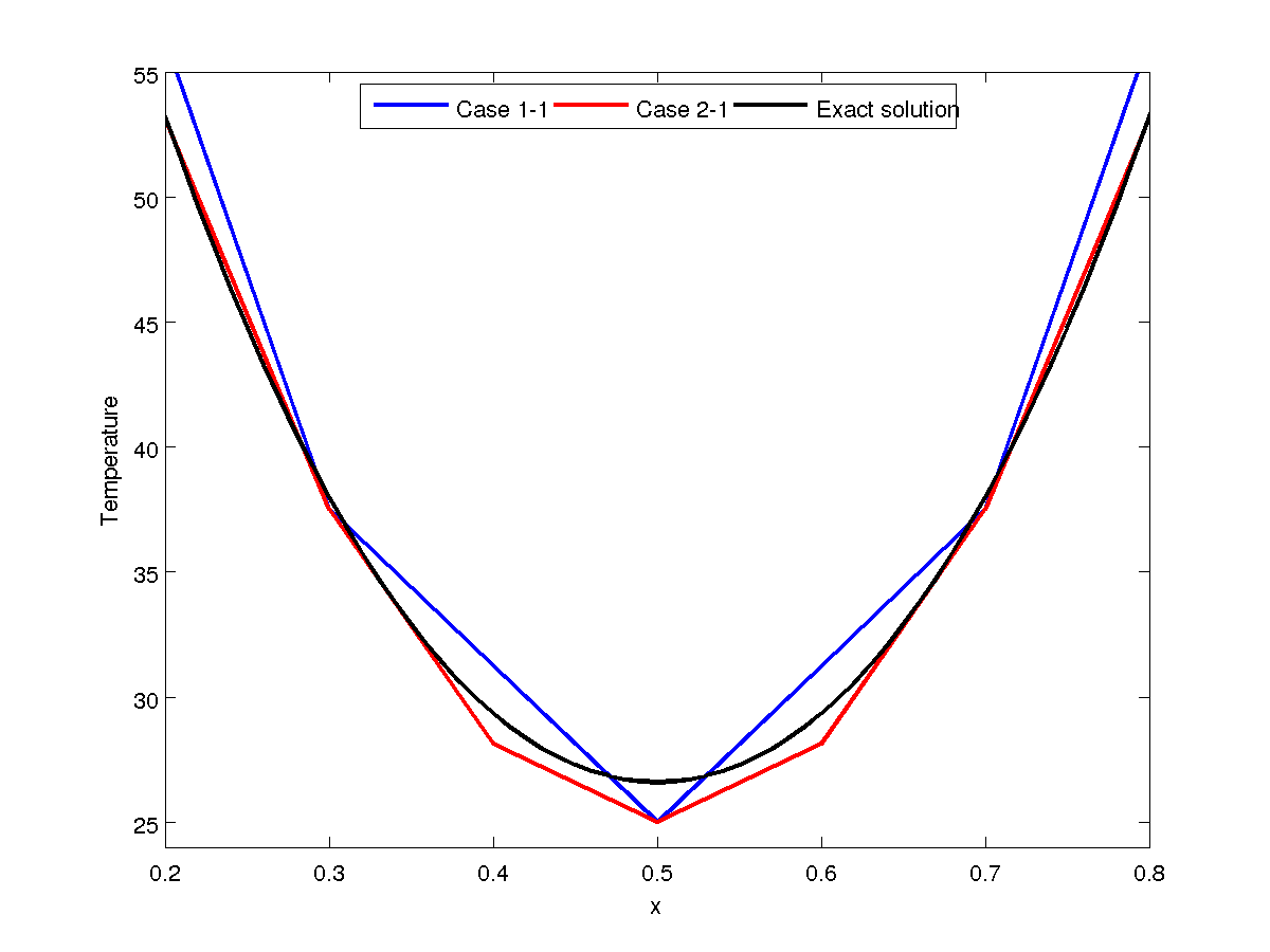
It is clear that the second case is more accurate even with such a course grid.
Moreover, the rms error could be obtained from:
\begin{equation} \text{RMS} = \sqrt{\left.\sum\limits_{j=1}^{J_{max}} (T_j - \text{TE}_j)^2 \right/ J_{max}.} \end{equation} Computing the rms error helps to compare two mentioned cases more accurately. This comparison will be done after computing the problem for different values of $ s $.
More accurate numerical solutions
Decreasing the value of $ s $ results in a more accurate solution. But also the results depend on $ \Delta x $ and $ \Delta t $ variations. It means that the magnitude of error would change for a fixed value of $ s $, but different combinations of $ \Delta x $ and $ \Delta t $. To show this, the second case (which seems to be more accurate than the first case) is modified as it is shown in Table b.3.1. A comparison of all cases is illustrated in this table.

As an example, comparing the rms error of cases (2-2) and (2-4) shows that although the value of $ s $ is decreased, the error is larger. Because the grid is not fine enough. Refining the grid in case (2-5) leads to a much better results. The following figures show the temperature distribution for some cases together with the exact solution.


Stability
Now it is easily possible to check the stability of the scheme by running the case (2-7) in which the value of $ s>0.5 $ makes it unstable. This is plotted in Fig. b.3.7 to show the unstable solution.

The relevant Matlab codes can be downloaded using the following link:
Matlab Codes Bank
No comments:
Post a Comment